Manipulation 赛道是官方提供baseline 模型,需要完成10项任务,每项任务的完成分为1分,总分10分,提交自己的模型,获得更高的分数。十个任务分别如下,提高的模型有两个:UniVLA 和RDT

智元的Genie Sim 环境是在NVIDIA ISAAC Sim基础上开发的机器人仿真平台,能够查看机器人在仿真环境中的任务表现。

具体的准备过程在这个链接: Genie Sim Benchmark
租用云服务器是很好的选择,如果自己购置GPU,一方面无法灵活配置,价格昂贵,另一方面安装环境也容易被折腾。云服务器随时取用,非常方面,我租用的平台是“智星云”,开始测试的时候用的RTX 4090, 可以选择多GPU和CPU 内存,后面训练的时候切换A100,可谓非常灵活。
租用的版本主要分三个阶段:
大模型训练的另一个特点是数据集非常庞大,一般都要在huggingface上下载,虽然用git 也行,但下载速度慢,且容易卡断。如果你遇到相同的问题,一定要看这篇知乎,加速效果异常好! 使用 HFD 加快 Hugging Face 模型和数据集的下载 仿真数据集将近1T,直接扩容硬盘到了2T。
wget https://hf-mirror.com/hfd/hfd.sh
chmod a+x hfd.sh
echo 'export HF_ENDPOINT=https://hf-mirror.com' >> ~/.bashrc
source ~/.bashrc
./hfd.sh gpt2 --tool aria2c -x 4
./hfd.sh agibot-world/AgiBotWorldChallenge-2025 --tool aria2c -x 4 --include Manipulation-SimData/*
按Genie Sim Benchmark的流程可以跑起仿真。期间有遇到几个问题
SIM_ASSETS=~/GenieSimAssets ./scripts/start_gui.sh
./scripts/autorun.sh iros_pack_in_the_supermarket infer UniVLA
报错信息:
这是terminal的问题,运行autorun.sh 脚本的时候,会遍历系统已有的terminal,首选是gnome_terminal,但我这边有些问题,调整成“terminator”之后就ok了。

还是在auto_run.sh 的脚本,它会通过terminator 运行三个任务:
脚本最后有个while 循环,会检测后台的任务,判断是否超时来退出仿真。我这边的仿真加载慢,经常被强制kill,最后索性注释退出机制,就能成功run起来!
模型训练卡了很久,需要下载额外下载依赖,添加配置。
按此步骤,不用安装Depth-Anything

这个库其实包含在仓库的InternVL 文件夹里,需要export 对应的路径

需要把Depth-Anything仓库的facebookresearch_dinov2_main 放到latent_action_model 目录下:

训练过程中需要加载这个权重,但原仓库下没有这个权重。

在hf 里面搜关键字,终于找到同名的模型权重!

README.md展示的只是示例,具体训练的时候需要修改
其中dataset 的结构如下,hf下载的数据集需要先解压,并放一起:

训练到了10%,后续异常退出。此时GPU内存48G,htop查看训练过程中CPU内存的使用量,发现才16G,远远不够!提高CPU 内存能够解决问题。
服务器CPU 内存的选取有限,为了不让cpu 内存爆掉导致训练终止,需要用其他方法提高内存,最有效的是提高swap分区的大小!后期训练的时候,直接把swap 分区提高到了300G,内存自由!
Linux系统swap分区扩容保姆级教程
univla 的训练效果和batch size 有很大关系,一般训练的标配都是8卡A100,每张卡80G,bs=8。然后训练5万步左右。
开始训的时候,我只有可怜的单卡,48G,bs=1,根本没法收敛,越训越烂。 训练的调整过程如下:
早期测试可以先提交官方的baseline模型,确认格式:解压之后直接是以下文件夹。

cd UniVLA
zip -r ../univla_ori.zip .
提交之后,训练显示size 不对。原因是训练的时候没有加 --wogripper 参数,但推理默认是开的,导致不匹配。机械臂包含7各自由度+夹爪1个自由度,双臂就有16个自由度,如果去除夹爪,就只有14个自由度。
解决方式有两种:
赛后八卦: 8卡GPU bs=8, UniVLA训练5万步,分数能到2.45左右 8卡GPU bs默认, RDT训练10万步,分数能到2.45左右 UniVLA 模型的训练好坏,和bs 关系很大,越大越好,调大grad_accumulation 可以增大bs,以时间换空间
]]>可以在pycharm找nn.Conv2d的定义文件,然后搜索‘reset_parameters’就可以看到它的初始化函数,
同理可以查看nn.BatchNorm2d,nn.Linear的初始化函数。
下面是简单的VGG网络示例
import torch
import torch.nn.functional as F
import troch.nn as nn
class VGG(nn.Module):
def __init__(self):
super(VGG, self).__init__()
self.conv1 = nn.Conv2d(3, 32, 3, 1, 1,bias=False)
self.conv2_1 = nn.Conv2d(32, 64, 3, 1, 1,bias=False)
self.conv2_2 = nn.Conv2d(64, 64, 3, 1, 1,bias=False)
self.conv3_1 = nn.Conv2d(64, 128, 3, 1, 1,bias=False)
self.conv3_2 = nn.Conv2d(128, 128, 3, 1, 1,bias=False)
self.conv3_3 = nn.Conv2d(128, 128, 3, 1, 1,bias=False)
self.fc1 = nn.Linear(2048, 128,bias=False)
self.fc2 = nn.Linear(128, 10,bias=False)
def forward(self, x):
out = F.relu(self.conv1(x))
out = F.max_pool2d(out, 2)
out = F.relu(self.conv2_1(out))
out = F.relu(self.conv2_2(out))
out = F.max_pool2d(out, 2)
out = F.relu(self.conv3_1(out))
out = F.relu(self.conv3_2(out))
out = F.relu(self.conv3_3(out))
out = F.max_pool2d(out, 2)
out = out.view(out.size(0), -1)
out = F.relu(self.fc1(out))
out = self.fc2(out)
return out
#定义初始化函数
def weights_init(m):
if isinstance(m, nn.Conv2d):
nn.init.constant_(m.weight, 0.5)
#nn.init.constant_(m.bias, 0)
#nn.init.kaiming_normal_(m.weight, mode='fan_out', nonlinearity='relu')
#nn.init.xavier_normal_(m.weight)
elif isinstance(m, nn.Linear):
nn.init.xavier_uniform_(m.weight)
#nn.init.constant_(m.bias,0)
net = VGG()
#apply函数会递归地搜索网络内的所有module并把参数表示的函数应用到所有的module上。
net.apply(weights_init)
# 显示网络参数字典的key
net.state_dict().keys()
# 输出conv1层卷积权重
net.state_dict()['conv1.weight']
]]>RK3399Pro NPU Manual提供了入门指导,里面的RKNN toolkit 包含了样例和转换工具。我的unet版本是参考github头像匹配的pytorch版本。
样例提供了torchvision上resnet_18的python版本,能够成功转成rknn格式,代码如下:
import numpy as np
import cv2
from rknn.api import RKNN
import torchvision.models as models
import torch
if __name__ == '__main__':
net = models.resnet_18(pretrained=True)
net.eval()
trace_model = torch.jit.trace(net, torch.Tensor(1, 3, 224, 224))
trace_model.save('./resnet_18.pt')
model = './resnet_18.pt'
input_size_list = [[3,224,224]]
# Create RKNN object
rknn = RKNN()
# pre-process config
print('--> config model')
rknn.config(channel_mean_value='123.675 116.28 103.53 58.395', reorder_channel='0 1 2')
print('done')
# Load pytorch model
print('--> Loading model')
ret = rknn.load_pytorch(model=model, input_size_list=input_size_list)
if ret != 0:
print('Load pytorch model failed!')
exit(ret)
print('done')
# Build model
print('--> Building model')
ret = rknn.build(do_quantization=False, dataset='./dataset.txt')
if ret != 0:
print('Build pytorch failed!')
exit(ret)
print('done')
# Export rknn model
print('--> Export RKNN model')
ret = rknn.export_rknn('./resnet_18.rknn')
if ret != 0:
print('Export resnet_18.rknn failed!')
exit(ret)
print('done')
这里有个关键函数,torch.jit.trace,JIT表示Just In Time Compilation,即时编译。它是Python和C++的桥梁,我们可以使用python训练模型,然后通过JIT将模型转为与语言无关的静态图,供C++调用,能非常方便得部署到树莓派、IOS、Android等设备。
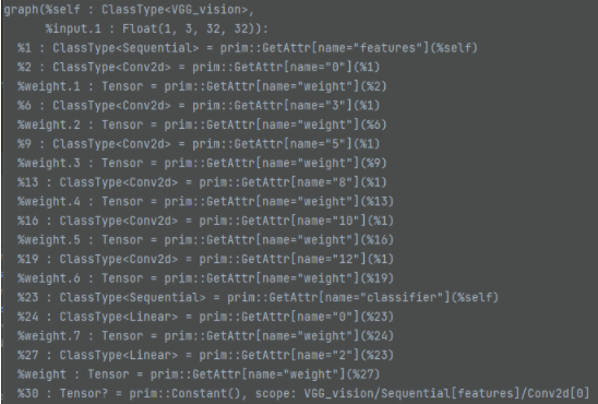
静态图大概长这样:

我一开始先想部署自己训练的VGG模型,网络尽量接近torchvision_models的样例,定义如下:
import torch.nn as nn
import torch
class VGG(nn.Module):
def __init__(self):
super(VGG, self).__init__()
self.conv1 = nn.Conv2d(3, 32, 3, 1, 1,bias=False)
self.relu = nn.ReLU(inplace=True)
self.conv2_1 = nn.Conv2d(32, 64, 3, 1, 1,bias=False)
self.max_pool2d = nn.MaxPool2d(kernel_size=2,stride=2)
self.conv2_2 = nn.Conv2d(64, 64, 3, 1, 1,bias=False)
self.conv3_1 = nn.Conv2d(64, 128, 3, 1, 1,bias=False)
self.conv3_2 = nn.Conv2d(128, 128, 3, 1, 1,bias=False)
self.conv3_3 = nn.Conv2d(128, 128, 3, 1, 1,bias=False)
self.fc1 = nn.Linear(2048, 128,bias=False)
self.fc2 = nn.Linear(128, 10,bias=False)
def forward(self, x):
out = self.relu(self.conv1(x))
out = self.max_pool2d(out)
out = self.relu(self.conv2_1(out))
out = self.relu(self.conv2_2(out))
out = self.max_pool2d(out)
out = self.relu(self.conv3_1(out))
out = self.relu(self.conv3_2(out))
out = self.relu(self.conv3_3(out))
out = self.max_pool2d(out)
out = torch.flatten(out,1)
out = self.relu(self.fc1(out))
out = self.fc2(out)
return out
结果奇怪的是,当运行到ret = rknn.load_pytorch(model=model, input_size_list=input_size_list),一直报错:
AttrubuteError:'NoneType' object has no attribute 'get_input_layers'
rknn.load_python函数是以动态库的方式给的,pycharm debug模式看不到源码,产看静态图,也找不到input_layers这种信息,为之奈何? 竟然官网的样例可以跑通,那一定是模型定义的问题,因此反复比较我的VGG模型和torchvision models上alexnet的区别,终于发现了,不同,虽然有点不理解,但最终还是跑通了:

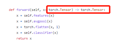
官网forward函数添加了输入输出类型的定义,torch.Tensor!?这还用定义?这不明摆的吗,真是服了。
跑通VGG,说明卷积、下采样等函数是支持的,Unet与之相比,只增加了两点:
unet模型定义如下:
import torch
import torch.nn as nn
class DoubleConv(nn.Module):
"""(convolution => [BN] => ReLU) * 2"""
def __init__(self, in_channels, out_channels):
super().__init__()
self.double_conv = nn.Sequential(
nn.Conv2d(in_channels, out_channels, kernel_size=3, padding=1),
nn.BatchNorm2d(out_channels),
nn.ReLU(inplace=True),
nn.Conv2d(out_channels, out_channels, kernel_size=3, padding=1),
nn.BatchNorm2d(out_channels),
nn.ReLU(inplace=True)
)
def forward(self, x:torch.Tensor)->torch.Tensor:
return self.double_conv(x)
class Down(nn.Module):
"""Downscaling with maxpool then double conv"""
def __init__(self, in_channels, out_channels):
super().__init__()
self.maxpool_conv = nn.Sequential(
nn.MaxPool2d(2),
DoubleConv(in_channels, out_channels)
)
def forward(self, x:torch.Tensor)->torch.Tensor:
return self.maxpool_conv(x)
class Up(nn.Module):
"""Upscaling then double conv"""
def __init__(self, in_channels, out_channels, bilinear=True):
super().__init__()
self.up = nn.Upsample(scale_factor=2, mode='bilinear', align_corners=True)
self.conv = DoubleConv(in_channels, out_channels)
#def forward(self, x1:torch.Tensor, x2:torch.Tensor)->torch.Tensor:
def forward(self, x: torch.Tensor) -> torch.Tensor:
x = self.up(x)
return self.conv(x)
class OutConv(nn.Module):
def __init__(self, in_channels, out_channels):
super(OutConv, self).__init__()
self.conv = nn.Conv2d(in_channels, out_channels, kernel_size=1)
def forward(self, x:torch.Tensor)->torch.Tensor:
return self.conv(x)
CHANNEL = 64
class UNet(nn.Module):
def __init__(self, n_channels, n_classes, bilinear=True):
super(UNet, self).__init__()
self.n_channels = n_channels
self.n_classes = n_classes
self.bilinear = bilinear
self.inc = DoubleConv(n_channels, CHANNEL)
self.down1 = Down(CHANNEL, CHANNEL * 2)
self.down2 = Down(CHANNEL * 2, CHANNEL * 4)
self.down3 = Down(CHANNEL * 4, CHANNEL * 8)
self.down4 = Down(CHANNEL * 8, CHANNEL * 8)
self.up1 = Up(CHANNEL * 16, CHANNEL * 4, bilinear)
self.up2 = Up(CHANNEL * 8, CHANNEL * 2, bilinear)
self.up3 = Up(CHANNEL * 4, CHANNEL, bilinear)
self.up4 = Up(CHANNEL * 2, CHANNEL, bilinear)
self.outc = OutConv(CHANNEL, n_classes)
def forward(self, x):
x1 = self.inc(x)
x2 = self.down1(x1)
x3 = self.down2(x2)
x4 = self.down3(x3)
x5 = self.down4(x4)
x = self.up1(x5, x4)
x = self.up2(x, x3)
x = self.up3(x, x2)
x = self.up4(x, x1)
logits = self.outc(x)
return logits
跨层拼接的其实可以参考resnet_18,将原来unet合并的up层展开为上采样+双层卷积,不是硬伤。 难点就在上采样函数,单独提取出来,转换上采样函数,一直报这样的错误:
int() argument must be a string , a bytes-like object or a number, not 'NoneType'
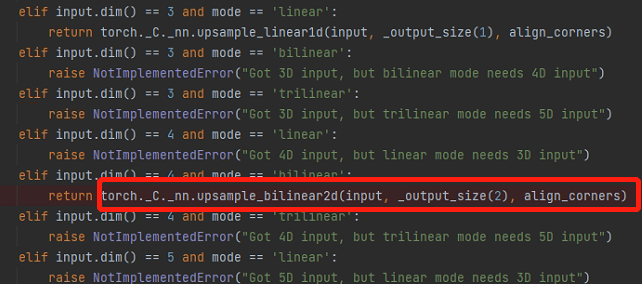
这是啥玩意,pycharm在debug模式下,终于找到torch.Upsample()最后调用的函数torch._C._nn.upsample_bilinear2d()

它会经过一系列判断,获得输入图的维度dim和尺寸信息,最后调用这个内嵌函数。然而,获取输出图像大小时,它调用了input.size()函数,这是报错的关键,静态图怎么要调用这个函数呢?输入确定的情况下,这个大小应该也是确定的吧,直接换成确定大小就行。

知道症结之后,针对跨层拼接和上采样,对模型稍加修改(输入特征图定为544x544):
""" Full assembly of the parts to form the complete network """
import torch
import torch.nn as nn
class DoubleConv(nn.Module):
"""(convolution => [BN] => ReLU) * 2"""
def __init__(self, in_channels, out_channels):
super().__init__()
self.double_conv = nn.Sequential(
nn.Conv2d(in_channels, out_channels, kernel_size=3, padding=1),
nn.BatchNorm2d(out_channels),
nn.ReLU(inplace=True),
nn.Conv2d(out_channels, out_channels, kernel_size=3, padding=1),
nn.BatchNorm2d(out_channels),
nn.ReLU(inplace=True)
)
def forward(self, x:torch.Tensor)->torch.Tensor:
return self.double_conv(x)
class Down(nn.Module):
"""Downscaling with maxpool then double conv"""
def __init__(self, in_channels, out_channels):
super().__init__()
self.maxpool_conv = nn.Sequential(
nn.MaxPool2d(2),
DoubleConv(in_channels, out_channels)
)
def forward(self, x:torch.Tensor)->torch.Tensor:
return self.maxpool_conv(x)
class OutConv(nn.Module):
def __init__(self, in_channels, out_channels):
super(OutConv, self).__init__()
self.conv = nn.Conv2d(in_channels, out_channels, kernel_size=1)
def forward(self, x:torch.Tensor)->torch.Tensor:
return self.conv(x)
CHANNEL = 64
INPUT_SIZE = 544
class UNet(nn.Module):
def __init__(self, n_channels, n_classes, bilinear=True):
super(UNet, self).__init__()
self.n_channels = n_channels
self.n_classes = n_classes
self.bilinear = bilinear
self.inc = DoubleConv(n_channels, CHANNEL)
self.down1 = Down(CHANNEL, CHANNEL * 2)
self.down2 = Down(CHANNEL * 2, CHANNEL * 4)
self.down3 = Down(CHANNEL * 4, CHANNEL * 8)
self.down4 = Down(CHANNEL * 8, CHANNEL * 8)
self.conv1 = DoubleConv(CHANNEL * 16, CHANNEL * 4)
self.conv2 = DoubleConv(CHANNEL * 8, CHANNEL * 2)
self.conv3 = DoubleConv(CHANNEL * 4, CHANNEL)
self.conv4 = DoubleConv(CHANNEL * 2, CHANNEL)
self.outc = OutConv(CHANNEL, n_classes)
def forward(self, x:torch.Tensor)->torch.Tensor:
x1 = self.inc(x)
x2 = self.down1(x1)
x3 = self.down2(x2)
x4 = self.down3(x3)
x = self.down4(x4)
x = torch._C._nn.upsample_bilinear2d(x, [INPUT_SIZE//8, INPUT_SIZE//8], True)
x = self.conv1(torch.cat([x4,x],dim=1))
x = torch._C._nn.upsample_bilinear2d(x, [INPUT_SIZE//4, INPUT_SIZE//4], True)
x = self.conv2(torch.cat([x3,x],dim=1))
x = torch._C._nn.upsample_bilinear2d(x, [INPUT_SIZE // 2, INPUT_SIZE // 2], True)
x = self.conv3(torch.cat([x2,x],dim=1))
x = torch._C._nn.upsample_bilinear2d(x, [INPUT_SIZE , INPUT_SIZE ], True)
x = self.conv4(torch.cat([x1,x],dim=1))
x = self.outc(x)
return x
这样就可以快乐的完成模型转换了!
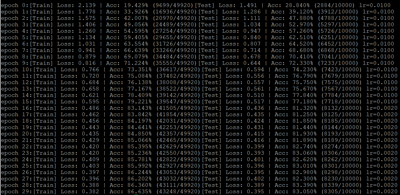
]]>设定学习率为0.01,训练30个epoch,batch_size=128。发现15个epoch之后训练变缓,因此可以在次改变学习率。最终的训练集86.1%,测试集集83.3%
#############1. 数据准备
import torch
import torch.nn as nn
import torch.nn.functional as F
from torchvision import transforms,datasets
datapath = '/home/Dataset/cifar10_data'
train_transform=transforms.Compose([
transforms.RandomCrop(32, padding=4),
transforms.RandomHorizontalFlip(),
transforms.ToTensor(),
transforms.Normalize((0.4914, 0.4822, 0.4465), (0.2023, 0.1994, 0.2010)),
])
test_transform=transforms.Compose([
transforms.ToTensor(),
transforms.Normalize((0.4914, 0.4822, 0.4465), (0.2023, 0.1994, 0.2010))
])
train_data= datasets.CIFAR10(root=datapath,train = True,transform = train_transform)
test_data = datasets.CIFAR10(root=datapath,train = False,transform =test_transform)
###############2.模型准备
class VGG(nn.Module):
def __init__(self):
super(VGG, self).__init__()
self.conv1 = nn.Conv2d(3, 32, 3, 1, 1,bias=False)
self.conv2_1 = nn.Conv2d(32, 64, 3, 1, 1,bias=False)
self.conv2_2 = nn.Conv2d(64, 64, 3, 1, 1,bias=False)
self.conv3_1 = nn.Conv2d(64, 128, 3, 1, 1,bias=False)
self.conv3_2 = nn.Conv2d(128, 128, 3, 1, 1,bias=False)
self.conv3_3 = nn.Conv2d(128, 128, 3, 1, 1,bias=False)
self.fc1 = nn.Linear(2048, 128,bias=False)
self.fc2 = nn.Linear(128, 10,bias=False)
def forward(self, x):
out = F.relu(self.conv1(x))
out = F.max_pool2d(out, 2)
out = F.relu(self.conv2_1(out))
out = F.relu(self.conv2_2(out))
out = F.max_pool2d(out, 2)
out = F.relu(self.conv3_1(out))
out = F.relu(self.conv3_2(out))
out = F.relu(self.conv3_3(out))
out = F.max_pool2d(out, 2)
out = out.view(out.size(0), -1)
out = F.relu(self.fc1(out))
out = self.fc2(out)
return out
net = VGG()
device = 'cuda' if torch.cuda.is_available() else 'cpu'
net = net.to(device)
from torchsummary import summary
summary(net,(3,32,32))
##############3.参数设置
epochs = 30
lr = 0.01
optimizer = torch.optim.SGD(net.parameters(), lr=lr, momentum=0.9, weight_decay=5e-4)
batch_size = 128
train_loader = torch.utils.data.DataLoader(train_data,batch_size=batch_size,shuffle=True,drop_last=True)
test_loader = torch.utils.data.DataLoader(test_data,batch_size=batch_size,shuffle=False,drop_last=False)
#################### 4.测试函数
def test():
net.eval()
test_loss = 0
correct = 0
total = 0
with torch.no_grad():
for batch_idx, (inputs, targets) in enumerate(test_loader):
inputs, targets = inputs.to(device), targets.to(device)
outputs = net(inputs)
loss = criterion(outputs, targets)
test_loss += loss.item()
_, predicted = outputs.max(1)
total += targets.size(0)
correct += predicted.eq(targets).sum().item()
#print('[Test] Loss: %.3f | Acc: %.3f%% (%d/%d) lr=%.4f' % (test_loss/(len(test_loader.dataset)/100), 100.*correct/total, correct, total,scheduler_warmup.get_lr()[0]))
print('[Test] Loss: %.3f | Acc: %.3f%% (%d/%d) lr=%.4f' % (test_loss/(len(test_loader.dataset)/100), 100.*correct/total, correct, total,lr))
####################5. 训练
net.train()
## Loss and optimizer
criterion = nn.CrossEntropyLoss()
best_acc =0
for epoch in range(epochs):
train_loss = 0
correct = 0
total = 0
print('epoch %d:'%(epoch),end="")
for batch_idx, (inputs, targets) in enumerate(train_loader):
inputs, targets = inputs.to(device), targets.to(device)
optimizer.zero_grad()
outputs = net(inputs)
loss = criterion(outputs, targets)
loss.backward()
optimizer.step()
train_loss += loss.item()
_, predicted = outputs.max(1)
total += targets.size(0)
correct += predicted.eq(targets).sum().item()
print('[Train] Loss: %.3f | Acc: %.3f%% (%d/%d)'% (train_loss/(batch_idx+1), 100.*correct/total, correct, total),end="")
test()
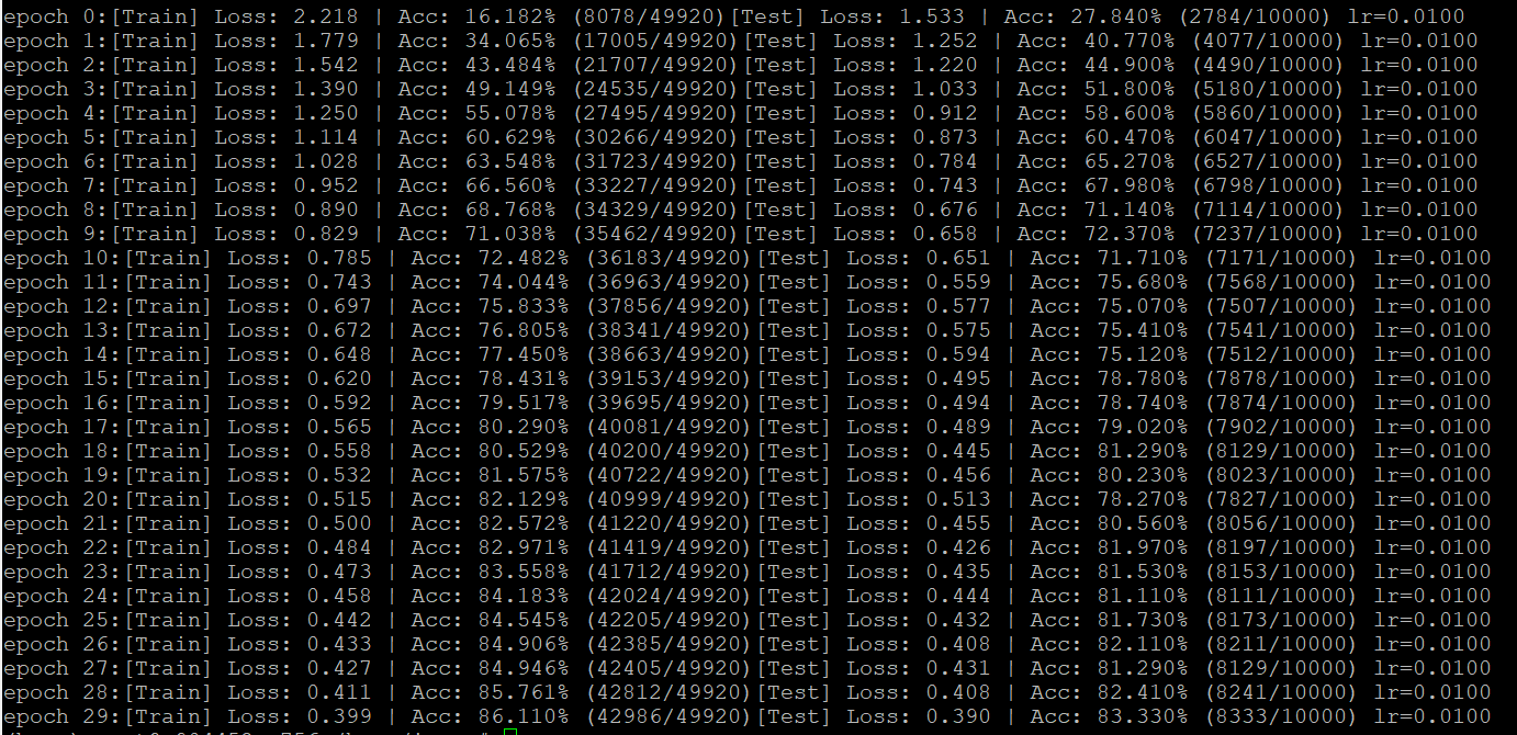
调整学习率需要导入'lr_scheduler'的包,调整选项,比如StepLR,ExpontialLR,MultiStepLR等,详情见链接。有实验表明,离散变化的学习率足以表现良好,首先用StepLR,需要修改三个地方: 1.参数设置部分
epochs = 30
# a.导入包
from torch.optim import lr_scheduler
lr = 0.01
optimizer = torch.optim.SGD(net.parameters(), lr=lr, momentum=0.9, weight_decay=5e-4)
#b.每16个epoch之后,lr变为原来的0.2
scheduler1 = lr_scheduler.StepLR(optimizer,step_size=16,gamma=0.2)
#scheduler1 = lr_scheduler.ExponentialLR(optimizer, gamma=0.95) # 每个epoch,lr变为原来的0.95
#scheduler1 = lr_scheduler.MultistepLR(optimizer,milestones=[10,20],gamma=0.5)# 10epoch后变为原来0.5,20 epoch后又衰减0.5
batch_size = 128
train_loader = torch.utils.data.DataLoader(train_data,batch_size=batch_size,shuffle=True,drop_last=True)
test_loader = torch.utils.data.DataLoader(test_data,batch_size=batch_size,shuffle=False,drop_last=False)
# c.通过scheduler1.get_lr()[0])查看当前学习率
print('[Test] Loss: %.3f | Acc: %.3f%% (%d/%d) lr=%.4f' % (test_loss/(len(test_loader.dataset)/100), 100.*correct/total, correct, total,scheduler1.get_lr()[0]))
#print('[Test] Loss: %.3f | Acc: %.3f%% (%d/%d) lr=%.4f' % (test_loss/(len(test_loader.dataset)/100), 100.*correct/total, correct, total,lr))
print('[Train] Loss: %.3f | Acc: %.3f%% (%d/%d)'% (train_loss/(batch_idx+1), 100.*correct/total, correct, total),end="")
test()
#d.调整学习率
scheduler1.step()
这是lr=0.01,scheduler1 = lr_scheduler.StepLR(optimizer,step_size=16,gamma=0.2)的结果,可见16个epoch减小学习率后,准确率从77% 跳到81%,再缓慢增加。
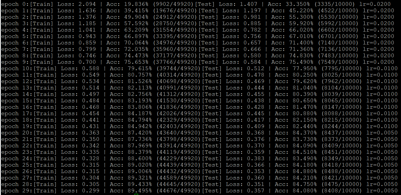
这是lr=0.02,scheduler1 = lr_scheduler.MultistepLR(optimizer,milestones=[10,20],gamma=0.5),可见第10、20epcoch处有2%的准确率跳变。
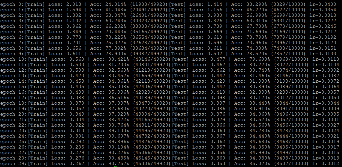
这是lr=0.04,scheduler1 = lr_scheduler.ExponentialLR(optimizer,gamma=0.885),30epoch 之后lr降为0.001。可见准确率增长相对稳定,最终到85%。
warmup 是学习率先快速增大,然后按之前设置的方式衰减,说明和用法在这,先安装warmup包pip install warmup-scheduler,然后也是修改三个地方:
epochs = 30
from torch.optim import lr_scheduler
#a.导入warmup包
from warmup_scheduler import GradualWarmupScheduler
lr = 0.001
optimizer = torch.optim.SGD(net.parameters(), lr=lr, momentum=0.9, weight_decay=5e-4)
#scheduler1 = lr_scheduler.StepLR(optimizer,step_size=10,gamma=0.2)
#scheduler1 = lr_scheduler.MultiStepLR(optimizer,milestones=[5,10,15,20,25],gamma=0.5)
#scheduler1 = lr_scheduler.ExponentialLR(optimizer, gamma=0.885)
#b.前5个epoch,从0.001增加到0.04,之后按scheduler1变化lr
scheduler_warmup = GradualWarmupScheduler(optimizer, multiplier=40, total_epoch=5, after_scheduler=scheduler1)
batch_size = 128
train_loader = torch.utils.data.DataLoader(train_data,batch_size=batch_size,shuffle=True,drop_last=True)
test_loader = torch.utils.data.DataLoader(test_data,batch_size=batch_size,shuffle=False,drop_last=False)
# c.通过scheduler_warmup.get_lr()[0])查看当前学习率
print('[Test] Loss: %.3f | Acc: %.3f%% (%d/%d) lr=%.4f' % (test_loss/(len(test_loader.dataset)/100), 100.*correct/total, correct, total,scheduler_warmup.get_lr()[0]))
#print('[Test] Loss: %.3f | Acc: %.3f%% (%d/%d) lr=%.4f' % (test_loss/(len(test_loader.dataset)/100), 100.*correct/total, correct, total,lr))
net.train()
## Loss and optimizer
criterion = nn.CrossEntropyLoss()
best_acc =0
for epoch in range(epochs):
#d.调整学习率
scheduler_warmup.step()
train_loss = 0
correct = 0
total = 0
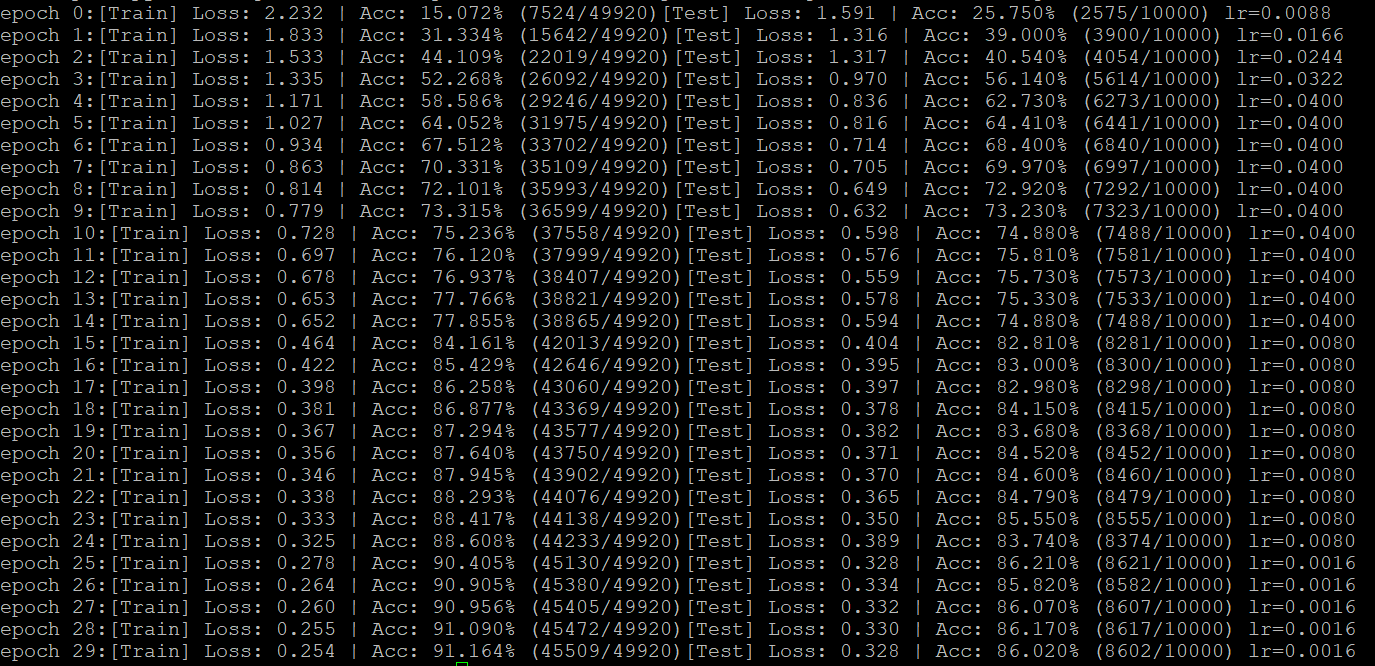
这是先warmup到0.4,再每10epoch缩小为原来的0.2。
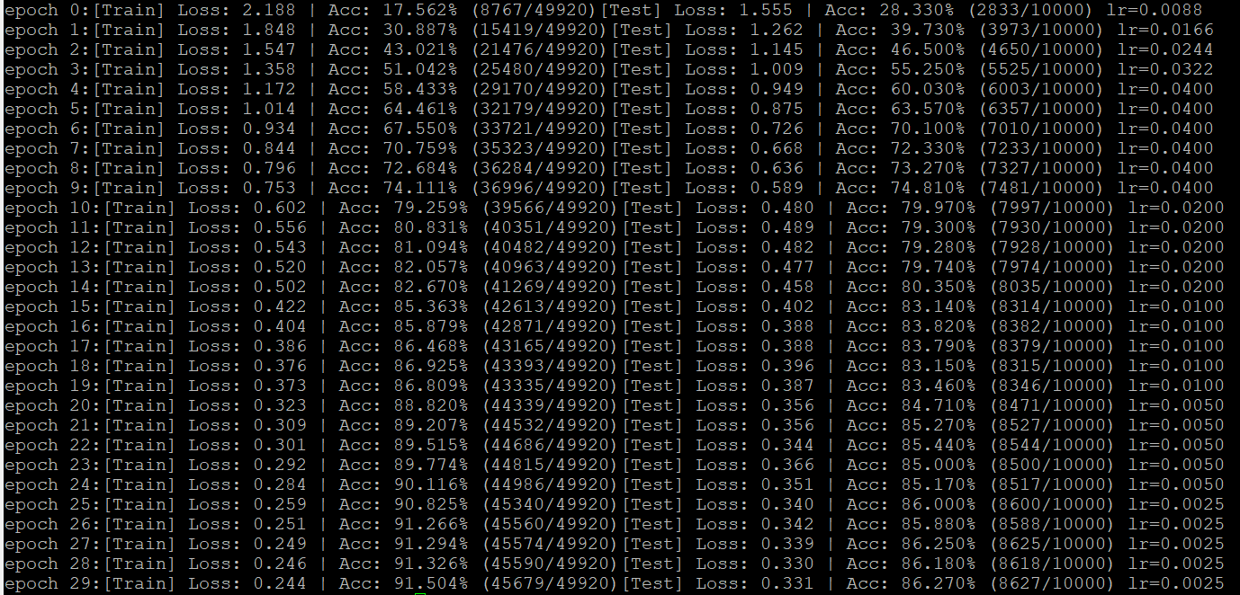
这是先warmup到0.4,在[5,10,15,20,25]的epoch节点上,缩小0.5。
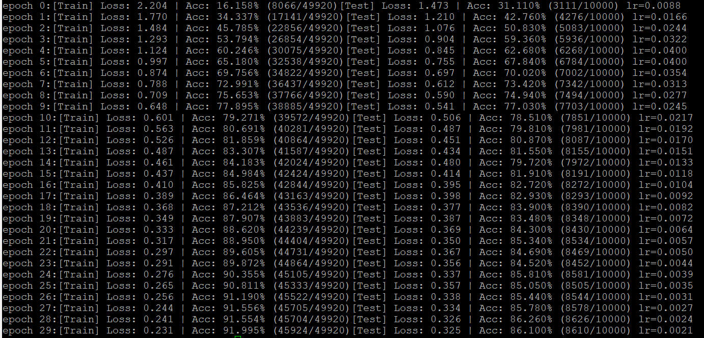
这是先warmup到0.4,每个epoch变为原来的0.885。
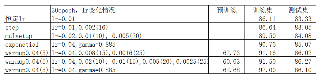
简单总结了一下上面的结果,调整学习率确实可以提升训练的效果,但要调好也不简单,比如batch_size,设为256时效果欠佳;比如起始学习率,0.01显然太小了。
最后附上代码:vgg_cifar10_lr_test.zip
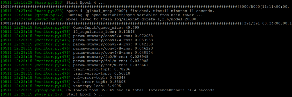
]]>svhn-digit-dorefa.py代码,这次准备跑alexnet-dorefa.py,其中碰到了无数的bug,折腾了好几天,终于跑通了!这里只挑选其中几个我花时间最多的bug。
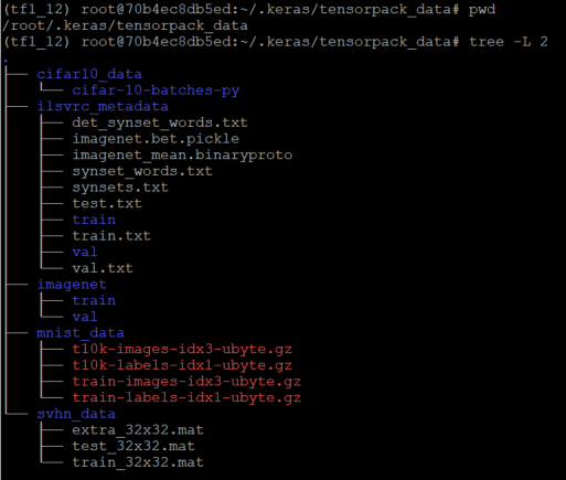
虽然官方代码有描述数据集路径,但对于脑残的我,还是不太理解,还是上图吧:

代码默认的目录是~/tensorpack_data/数据集,跑alexnet-dorefa.py的--data路径就是:/root/.keras/tensorpack_data/imagenet/
按如下代码运行:
python alexnet-dorefa.py --data /root/.keras/tensorpack_data/imagenet/ --dorefa 1,2,6 --gpu 0,1
出现Registered devices: [CPU, XLA_CPU, XLA_GPU]错误,感觉和硬件有关,参考这篇文章,说单GPU训练的时候是可以的,多GPU训练会碰到,于是为了先跑通,将--gpu 0,1改为--gpu 0。结果确实通过了,然后有了新的错误:
Default MaxPoolingOp only supports NHWC on device type CPU
搜了好久,才在tensorpack的论坛上找到原因,原来确实是GPU的问题,可以通过如下代码验证:
from tensorflow.python.client import device_lib
print(device_lib.list_local_devices())
结果确实发现少了库,报错是确实动态库:
libcublas.so.10.0: cannot open shared object file: No such file or directory
原来我的tensorflow是1.14.0版本,需要cuda10.0版本,对应的cudnn7.4.2版本。一开始还想上官网装cuda,又会是繁琐的工程,没想到可以借助conda快速配置环境:
conda install cudatoolkit=10.0
conda install cudnn=7.4
神经网络快把我变神经病了,配置环境花了那么多时间!看似简简单单的几条命令,背后却是满满的辛酸泪。。。 python,tensorflow,cuda,cudnn版本官方对照 这下终于可以运行了:
python alexnet-dorefa.py --data /root/.keras/tensorpack_data/imagenet/ --dorefa 1,2,6 --gpu 0,1
nvidia-smi -L #可以查看可以调用GPU的编号
上图纪念一番:

tensorflow,pytorch 等框架下也有量化操作,通常是为了减少权重存储空间,有利于部署移动端。但是基于数字电路的量化只能是均匀的,那么为什么还要研究非均匀量化呢?
忆阻器的电导权重是模拟量,本身具备非均匀量化的可能性,而且忆阻器电导的中间值比较不稳定,均匀量化的时候很难精确。
神经网络的权重本身是非均匀分布的,在密集的地方多取点,稀疏的地方少取点,量化后的误差会更小。

选取的量化点有一个中心思想:它们最接近原始的分布。正好,数学上有个“反变换采样定理”:
假设$U~(0,1)$均匀分布,Y为任意随机变量,$F_Y(y)$为Y的分布,$F^{-1}_Y(y)$为其反函数,则$Z=F_Y^{-1}(U)$与Y同分布。
Inverse transform sampling - Wikipedia

上面的公式很抽象,直接看左图吧。首先想个问题:如果只有一个(0,1)区间均匀随机数发生器,该如何通过变换,生成高斯分布?
我们可以求出高斯分布的分布函数,如中间的曲线,然后每产生(0,1)的随机数,作为纵坐标,确定对应的横坐标,即为高斯随机数。采样5万次之后,会有左图下边的分布。这样就通过分布函数,建立了均匀分布和任意分布的一一映射关系。
接下来的问题是,对任意分布做量化,使其最接近原始分布。我们可以求出统计出分布函数,再映射到均匀分布,之后对均匀分布做量化,最后将量化的结果反映射到原分布,即可确定非均匀量化点。
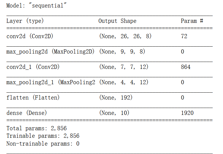
网络为两层卷积,分别8、12个通道,无bias;一层全连接,无bias。

非均匀量化

均匀量化

简单量化

网络为两卷积,分别32、64个通道,无bias;一层全连接,无bias。

非均匀量化

均匀量化

简单量化

上述结果容易看出,非均匀量化在level数更低的时候有更强的鲁棒性,确实效果会好一些。
但老师说4level量化之后精度还是掉很多,二值网络都可以到95%的精度。我确实惊呆了,怎么做到的!
接下来的任务是复现BNN网络,看看二值网络到底如何训练和推理;然后学习LLoyd在脉冲调制中最小二乘法量化方案。
]]># 1.数据准备
import tensorflow as tf
import numpy as np
mnist = tf.keras.datasets.mnist
img_rows,img_cols = 28,28
(x_train_, y_train_), (x_test_, y_test_) = mnist.load_data()
x_train = x_train_.reshape(x_train_.shape[0],img_rows,img_cols,1)
x_test = x_test_.reshape(x_test_.shape[0],img_rows,img_cols,1)
x_train = x_train.astype('float32')
x_test = x_test.astype('float32')
x_train = x_train / 256
x_test = x_test / 256
y_train_onehot = tf.keras.utils.to_categorical(y_train_)
y_test_onehot = tf.keras.utils.to_categorical(y_test_)
model = tf.keras.Sequential()
model = tf.keras.models.load_model('models/mnist_tf2_fw.h5')
score = model.evaluate(x_test, y_test_onehot, verbose=0)
print('Test accuracy:', "{:.5f}".format(score[1]))
interpreter= tf.lite.Interpreter(model_path="models/tflite_tf2_8.tflite")
#interpreter= tf.lite.Interpreter(model_path="models/tflite_tf2_dy.tflite")
#interpreter= tf.lite.Interpreter(model_path="models/tflite_tf2_16.tflite")
#interpreter= tf.lite.Interpreter(model_path="models/tflite_tf2_32.tflite")
interpreter.allocate_tensors()
input_details=interpreter.get_input_details()
output_details=interpreter.get_output_details()
#print(input_details)
#print(output_details)
y_lebal=y_test_onehot.argmax(1)
# 量化模型推理
pre = []
# tflite针对安卓端运用,每次只能推理一个数据
for i in range (len(x_test)):
# .astpe 非常重要,找了很久才解决这个bug
x_test1 = x_test[i].reshape(1,28,28,1).astype(np.float32)
interpreter.set_tensor(input_details[0]['index'],x_test1)
interpreter.invoke()
output_data = interpreter.get_tensor(output_details[0]['index'])
pre.append(output_data.argmax())
temp = (pre==y_lebal)
acc=sum(temp)/10000
print(acc)
| 32bit | 16bit | 8bit | 默认 |
|---|---|---|---|
| 98.500 | 98.500 | 98.440 | 98.440 |
这结果似乎和权重量化的差不多。数据流量化确实不太容易,需要更加底层、细粒度的操作。只有rram的训练有可能是4bit和8bit的混合,所以低精度数据流的训练还是挺重要的。
后期计划,做低比特、数据流量化的调用,看看别人的工作,为rram高性能计算打下理论基础。 github 代码
]]># 1. 加载数据集
import tensorflow as tf
import numpy as np
minst = tf.keras.datasets.mnist
img_rows,img_cols = 28,28
(x_train, y_train), (x_test, y_test) = minst.load_data()
x_train = x_train.reshape(x_train.shape[0],img_rows,img_cols,1)
x_test = x_test.reshape(x_test.shape[0],img_rows,img_cols,1)
x_train = x_train.astype('float32')
x_test = x_test.astype('float32')
x_train = x_train / 255
x_test = x_test / 255
y_train_onehot = tf.keras.utils.to_categorical(y_train)
y_test_onehot = tf.keras.utils.to_categorical(y_test)
# 2. 加载模型和权重,测试准确率
model = tf.keras.Sequential()
model = tf.keras.models.load_model('models/mnist_tf2_fw.h5')
score = model.evaluate(x_test, y_test_onehot, verbose=0)
print('Test accuracy:', "{:.5f}".format(score[1]))
model = tf.keras.models.load_model('models/mnist_tf2_fw.h5')
# 这里0,2,5层分别表示conv1,conv2,fc层的权重
for i in [0,2,5]:
# 通过get_weights 和setweights修改权重
temp = model.layers[i].get_weights()[0]
# 0.15表征噪声的标准差
temp = temp + np.random.rand(*temp.shape)*0.15
model.layers[i].set_weights([temp])
score = model.evaluate(x_test, y_test_onehot, verbose=0)
print('Test accuracy:', "{:.5f}".format(score[1]))
# 8bit量化
bit = 8
model = tf.keras.models.load_model('models/mnist_tf2_fw.h5')
# 这里0,2,5层分别表示conv1,conv2,fc层的权重
for i in [0,2,5]:
temp = model.layers[i].get_weights()[0]
temp = np.rint(temp * np.power(2,bit))/np.power(2,bit)
model.layers[i].set_weights([temp])
score = model.evaluate(x_test, y_test_onehot, verbose=0)
print('Test accuracy:', "{:.5f}".format(score[1]))
统计结果如下:
| 噪声标准差 | 0 | 0.04 | 0.06 | 0.08 | 0.09 | 0.10 | 0.16 |
|---|---|---|---|---|---|---|---|
| 准确率 | 98.500 | 96.870 | 92.590 | 87.510 | 78.590 | 70.180 | 52.800 |
| 量化精度 | 32bit | 16bit | 8bit | 4bit | 3bit | 2bit | 1bit |
|---|---|---|---|---|---|---|---|
| 准确率 | 98.500 | 98.500 | 98.490 | 98.410 | 97.380 | 89.400 | 66.250 |
特别说明的是:这里只是对权重做量化,推理计算过程中的数据还是32bit的浮点数,所以结果上看,3bit量化的精度下降不多,只有约1%。
有意思的一点是:3bit量化的准确率和0.04噪声接近;2bit量化准确率和0.08噪声相近,1bit量化的准确率和0.16的噪声相当。
分析原因:3bit量化相当于最小精度是0.125,可以将其等效为$3\sigma$的偏差,求得标准差为0.041,即为0.04的噪声。
]]>还是那片nature的文章Fully hardware-implemented memristor convolutional neural network。忆阻器的精度很低,虽然外围的ADC是8bit,但忆阻器实际的精度有4bit就不错了。希望先用32bit浮点数训练网络,然后做量化,比较准确率的下降情况:
测试的环境如下:
python 3.7.4, tensorflow 2.0.0
import tensorflow as tf
import numpy as np
# 1.数据集准备
minst = tf.keras.datasets.mnist
img_rows,img_cols = 28,28
(x_train, y_train), (x_test, y_test) = minst.load_data()
# 卷积运算需要将原来的(6000,28,28)变成(6000,28,28,1) ,即增加通道的参数
x_train = x_train.reshape(x_train.shape[0],img_rows,img_cols,1)
x_test = x_test.reshape(x_test.shape[0],img_rows,img_cols,1)
# 需要将原来的0-255的整数转为32bit单精度浮点数,再归一化为[0,1]
x_train = x_train.astype('float32')
x_test = x_test.astype('float32')
x_train = x_train / 255
x_test = x_test / 255
# 标签为独热码的形式,方便交叉熵运算
y_train_onehot = tf.keras.utils.to_categorical(y_train)
y_test_onehot = tf.keras.utils.to_categorical(y_test)
keras搭建模型很方便:
# 2. 模型搭建
model = tf.keras.Sequential()
# 注意这里padding的类型“valid”,表示不填充外围,输出shape为(26,26,8)。并且没有设置bias,因为忆阻器硬件里不好添加
model.add(tf.keras.layers.Conv2D(8, kernel_size=(3, 3),padding="valid", activation='relu',use_bias=False,input_shape=(28, 28, 1)))
# 同样注意这里的padding类型“sample”,表示除不尽须填充而不是舍去,输出shape为(9,9,8)
model.add(tf.keras.layers.MaxPooling2D(pool_size=(3, 3),padding="same"))
# 同理,注意padding,输出shape=(7,7,12)
model.add(tf.keras.layers.Conv2D(12, kernel_size=(3, 3),padding="valid", activation='relu',use_bias=False,))
# 同理,注意padding,输出shape=(4,4,12)
model.add(tf.keras.layers.MaxPooling2D(pool_size=(2, 2),padding="same"))
model.add(tf.keras.layers.Flatten())
model.add(tf.keras.layers.Dense(10, use_bias=False,activation='softmax'))
model.summary()

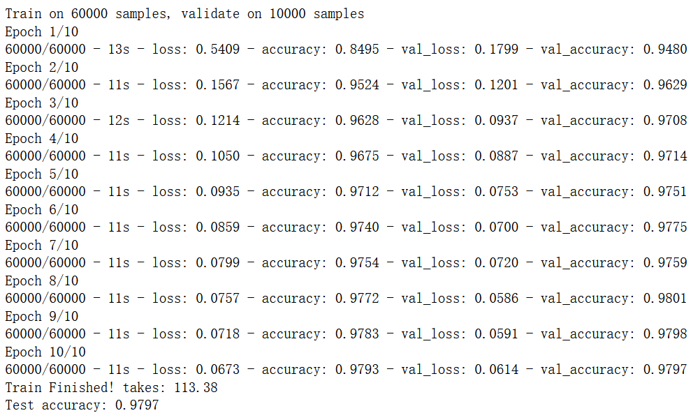
开始训练,数据集很小,cpu训练一两分钟左右就能达到98%准确率
model.compile(optimizer='adam', loss='categorical_crossentropy', metrics=['accuracy'])
from time import time
startTime = time()
history = model.fit(x_train, y_train_onehot, batch_size = 100, epochs = 10, verbose=2, validation_data = (x_test, y_test_onehot))
duration = time()-startTime
print("Train Finished! takes:","{:.2f}".format(duration))
score = model.evaluate(x_test, y_test_onehot, verbose=0)
print('Test accuracy:', score[1])

如果还要后续操作,模型的保存和加载还是相当重要的。
# 1.保存框架,权重,优化器,损失函数
model.save('models/mnist_tf2_fw.h5')
# 2.保存框架,不含权重和配置
yaml_tring = model.to_yaml()
with open('./models/mnist_tf2_f.yaml','w') as model_file:
model_file.write(yaml_tring)
# 3.保存权重,不含框架和配置
model.save_weights('models/mnist_tf2_w.h5')
保存量化后的tflite格式,找了好久才搞定的!tflite格式主要是为了安卓端推理应用推出的:
#1 未量化-32bit
converter = tf.lite.TFLiteConverter.from_keras_model(model)
tflite_model = converter.convert()
open("models/tflite_model_32.tflite","wb").write(tflite_model)
# 2.float16量化
converter = tf.lite.TFLiteConverter.from_keras_model(model)
converter.optimizations = [tf.lite.Optimize.DEFAULT]
converter.target_spec.supported_types = [tf.float16]
tflite_model = converter.convert()
open("models/tflite_model_16.tflite", "wb").write(tflite_model)
# 3.8bit量化
def representative_data_gen():
# *这里需要注意:函数需要获得x_train的shape信息
data = tf.data.Dataset.from_tensor_slices(x_train).batch(1).take(100)
for input_value in data:
yield [input_value]
converter = tf.lite.TFLiteConverter.from_keras_model(model)
converter.optimizations = [tf.lite.Optimize.DEFAULT]
converter.representative_dataset = representative_data_gen
# Restricting supported target op specification to INT8
converter.target_spec.supported_ops = [tf.lite.OpsSet.TFLITE_BUILTINS_INT8]
# Set the input and output tensors to uint8
converter.inference_input_type = tf.uint8
converter.inference_output_type = tf.uint8
# Convert and Save the model
tflite_model = converter.convert()
open("models/tflite_model_8.tflite", "wb").write(tflite_model)
# 4.动态量化
converter = tf.lite.TFLiteConverter.from_keras_model(model)
converter.optimizations = [tf.lite.Optimize.DEFAULT]
tflite_model = converter.convert()
open("models/tflite_model_dy.tflite", "wb").write(tflite_model)
截止目前,我们已经做好了训练,分别保存了32bit、16bit、8bit的量化模型。接下来的工作是加载模型,查看增加噪声、量化后对精度的损失。
]]>